Module 1: Crime Analysis
Part C of the Module 1 assignment was to create hotspot analysis of homicides in the City of Chicago using three different methods. All three methods would utilize a point feature class of the total homicides for 2017 and the City of Chicago boundary. A second feature class of the total homicides for 2018 would then be used to see how well the hotspot predicted the location of homicides.
Grid-based thematic mapping
This method utilized feature classes
for the total homicides for 2017, the City of Chicago boundary, and a ½ mile
grid cell clipped to the Chicago boundary. All three feature classes were added
to a map. The Spatial Join tool
was used to create a new feature class that would contain the count of
homicides for each grid cell. The Select By Attribute tool
was used to select only the cells where the number of homicides was greater
than 0. Next, the count column was sorted and the top 20% was selected and then
exported to a new feature class. The final feature class was dissolved to
create a single polygon for the hotspots.
Kernal Density
This method utilized feature classes
for the total homicides for 2017 and the City of Chicago boundary. The Kernel
Density tool was used to create a grid with cell size of 100 square miles.
Local Moran’s I
The last method
utilized feature classes for the total homicides for 2017, the City of Chicago
boundary, and the Census tracts polygons for the Chicago area. The Spatial
Join tool was used to create a new feature class that includes the homicide
counts in each of the census tract polygons. A new crime rate field was added
to the attribute table and the rate was calculated using the below formula:
!Join_Count! / !total_households! * 1000
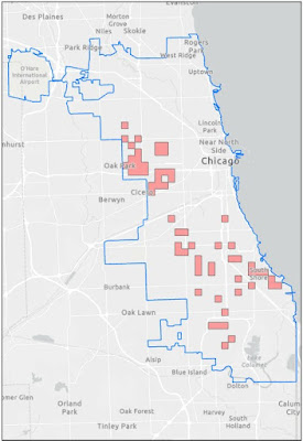
The Cluster and Outlier Analysis tool was then used to determine the significant clusters of high crime. A SQL query was performed to select just the high-high clusters features. The selected features were exported to a new feature class and a dissolve was performed to create a single hotspot polygon.
The Kernel
Density hotspot polygon contained 73% of the 2018 homicides but also the
largest area. This would probably not be the best choice to present to the police
chief. The Local Moran’s I hotspot polygon contained 45% of the 2018 homicides
and would be my recommendation since it less area for the police force to
cover.


Comments
Post a Comment